Calculus of Variations and Optimal Control:

Basic Concepts

1.Function and Functional

2.Increment of a function and functional

3.Differential of a Function

4.Variation of a Functional

5.Optimum function and Functional

Function:

A variable x is said to be a function of another variable t if, for every value of t in a given range, there exists a unique corresponding value of x. This relationship is written as:

x(t) = f(t)

This means there is a rule or correspondence that assigns to each value of t exactly one value of x.

Note: The variable t is often time, but it can represent any independent variable, such as distance, temperature, or spatial coordinates.

Examples:

1. x(t) = 2t² + 1
2. x(t) = 2t
3. x(t₁, t₂) = t₁³ + t₂²

In Example 3, x is a function of two independent variables, t₁ and t₂.

Functional:

A functional is a rule that assigns a single number to a function. If a quantity I depends on a function f(x), we write:

I = I(f(x))

This means that to each function f(x), there corresponds a specific number I. Unlike a function (which maps numbers to numbers), a functional maps functions to numbers.

Note: A functional may also depend on more than one function.

Example:

Let:

x(t) = 2t² + 1

Then the functional I is defined as:

I(x) = ∫₀¹ x(t) dt = ∫₀¹ (2t² + 1) dt

Evaluating the integral:

I = [ (2t³)/3 + t ]₀¹ = 2/3 + 1 = 5/3

Increment of a Function:

The increment of a function f, denoted by Δf, is defined as:

Δf ≈ f(t + Δt) − f(t)     (1.21)

This represents the change in the function’s value when the independent variable t changes by a small amount Δt.

Note: The increment Δf depends on both the value of t and the increment Δt.

Example 3:

Find the increment of the function:
f(t) = (t₁ + t₂)²

Solution:

Using the definition of increment:

Δf ≈ f(t + Δt) − f(t)

Substitute the values:

Δf = (t₁ + Δt₁ + t₂ + Δt₂)² − (t₁ + t₂)²

Expand the expression:

Δf = 2(t₁ + t₂) Δt₁ + 2(t₁ + t₂) Δt₂ + (Δt₁)² + (Δt₂)² + 2 Δt₁ Δt₂

This gives the approximate change in f due to small changes in t₁ and t₂.

So, the functional I maps the function x(t) = 2t² + 1 to the value 5/3.

Increment of a Functional

The increment of a functional I, denoted by ΔI, is defined as:

ΔI ≈ I(x(t) + δx(t)) – I(x(t))       (1.22)

Here, δx(t) is called the variation of the function x(t).

Since the increment of a functional depends on both the function x(t) and its variation δx(t), we write it as:

ΔI = ΔI(x(t), δx(t))

Example 4:

Find the increment of the functional:

I = ∫₀^t_f [2x²(t) + 1] dt

Solution:

ΔI ≈ I(x(t) + δx(t)) – I(x(t))

= ∫₀^t_f [2(x(t) + δx(t))² + 1] dt – ∫₀^t_f [2x²(t) + 1] dt

= ∫₀^t_f [4x(t)δx(t) + 2(δx(t))²] dt

Thus, the increment of the functional is:

ΔI = ∫₀^t_f [4x(t)δx(t) + 2(^]()

 Differential of a Function:

Let us define the increment of a function f at a point t^* as:

Δf ≈ f(t^* + Δt) − f(t^*)          (1.23)

Expanding f(t^* + Δt) about t^* using Taylor series, we get:

Δf = f(t^*) + (df/dt)_t=t^* Δt + (1/2!) (d²f/dt²)_t=t^* (Δt)² + higher order terms (h.o.t.) − f(t^*)

Simplifying, we get:

Δf ≈ (df/dt) Δt + (1/2!) (d²f/dt²) (Δt)² + …

The first term, (df/dt) Δt, is called the differential of the function f and is denoted by df.

Thus,

df = (df/dt) Δt

2. Differential as First-Order Approximation

Neglecting the higher-order terms in Δt (assuming Δt is very small), the increment of the function f becomes:

Δf ≈ (df/dt) · Δt = ḟ(t^*) · Δt = df · Δt          (1.24)

Here, df is called the differential of the function at the point t^*, and ḟ(t^*) is the derivative or slope of f at t^*.

In other words, the differential df provides a first-order (linear) approximation of the increment Δf of the function f.

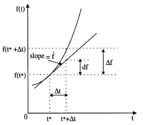
Fig.1 Increment Δf, Differential df, and Derivative f ̇(t) of a Function f( t)

Example 5:

Find the increment and the derivative of the function f(t) = t² + 2t.

Solution:

By definition, the increment Δf is:

Δf ≈ f(t + Δt) − f(t) = (t + Δt)² + 2(t + Δt) − (t² + 2t)

By Taylor series expansion:

= [t + 1·Δt + …]² + 2[t + 1·Δt + …] − (t² + 2t)

= t² + 2t·Δt + (Δt)² + 2t + 2Δt − (t² + 2t)

= 2t·Δt + 2Δt + higher order terms (neglected)

= 2(t + 1)·Δt

= 𝑓̇(t)·Δt

Therefore, increment Δf = 2(t + 1)·Δt = 𝑓̇(t)·Δt, and

Derivative: 𝑓̇(t) = 2(t + 1)

Variation of a Functional

The increment (or variation) of a functional is given by:

ΔI ≈ I(x(t) + δx(t)) − I(x(t))

Expanding I(x(t) + δx(t)) using Taylor series around x(t), we get:

ΔI = I(x(t)) + (∂I/∂x)·δx(t) + (1/2!)·(∂²I/∂x²)·(δx(t))² + … − I(x(t))

Simplifying:

ΔI = (∂I/∂x)·δx(t) + (1/2!)·(∂²I/∂x²)·(δx(t))² + …

Thus,

ΔI = δI + δ²I + … (1.25)

Where:

• δI is the first variation (linear in δx(t)),
• δ²I is the second variation (quadratic in δx(t)),
• Higher-order terms are neglected when δx(t) is small.

δI = (∂I/∂x) · δx(t),    δ²I = (1/2!) · (∂²I/∂x²) · [δx(t)]²

These are called the first variation (or simply the variation) and the second variation of the functional I, respectively.

The variation δI of a functional I is the linear (or first-order approximate) part (in δx(t)) of the increment ΔI.

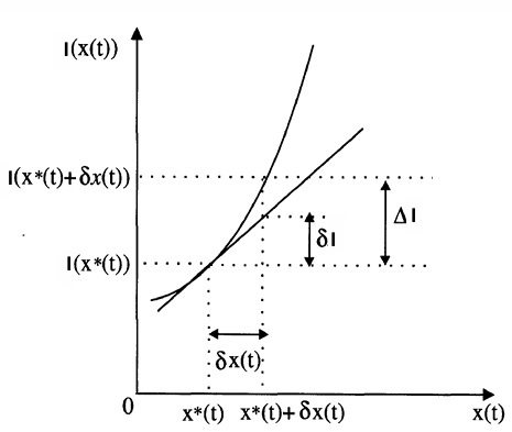
Fig. Increment ΔI  and the First Variation δI of the Functional J

Example 6:

Given the functional I(x(t)) = ∫_t₀^t_f [2x²(t) + 3x(t) + 4] dt, evaluate the variation of the functional.

Solution:

First, we form the increment and then extract the variation as the first-order approximation.

ΔI ≅ I(x(t) + δx(t)) − I(x(t))

= ∫_t₀^t_f [2(x(t) + δx(t))² + 3(x(t) + δx(t)) + 4] dt − ∫_t₀^t_f [2x²(t) + 3x(t) + 4] dt

= ∫_t₀^t_f [2(x(t)² + δx(t)² + 2x(t)·δx(t)) + (3x(t) + 3δx(t)) + 4] dt − ∫_t₀^t_f [2x²(t) + 3x(t) + 4] dt

= ∫_t₀^t_f [2x²(t) + 2δx²(t) + 4x(t)·δx(t) + 3x(t) + 3δx(t) + 4] dt − ∫_t₀^t_f [2x²(t) + 3x(t) + 4] dt

= ∫_t₀^t_f [2δx²(t) + 4x(t)·δx(t) + 3δx(t)] dt

Considering only the first-order terms (neglecting δx²(t)), we get the first variation:

δI(x(t), δx(t)) = ∫_t₀^t_f [4x(t) + 3] · δx(t) dt

Optimum Function

Definition: A function f(t) is said to have a relative optimum at the point t^* if there exists a positive parameter ε, such that for all points t in a domain D that satisfy |t − t^*| < ε, the increment of f(t) has the same sign (positive or negative).

If Δf(t) = f(t) − f(t^*) ≥ 0, then f(t^*) is a relative local minimum.

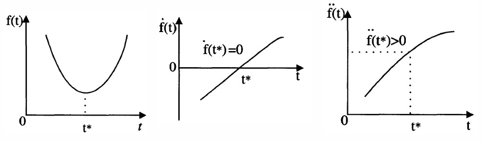
Fig. Minimum of a function

If Δf(t) = f(t) – f(t^*) ≤ 0, then f(t^*) is a relative local maximum.

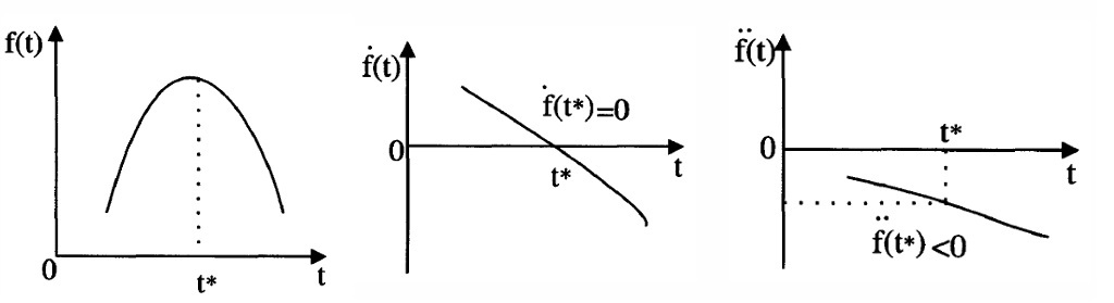
Fig. Maximum of a function

Global Optimum and Conditions for Optimality

If the previous relations hold for arbitrarily large values of 𝜖, then the function f(t^*) is said to have a global (absolute) optimum.

It is well known that a necessary condition for optimality of a function is that the first differential vanishes, i.e.,

df = 0

Sufficient Conditions:

• For a minimum, the second differential must be positive:
  d²f > 0
• For a maximum, the second differential must be negative:
  d²f < 0
• If d²f = 0, then the point is a stationary point, which may be an inflection point.

Analogous to finding extremum or optimal values for functions, in variational problems involving functionals, the result is that the variation must be zero on an optimal curve.

Let us now state this result as a theorem, known as the Fundamental Theorem of the Calculus of Variations.

Theorem:

For x^*(t) to be a candidate for an optimum, the first variation of I must be zero on x^*(t), i.e.,

δI(x^*(t), δx(t)) = 0 for all admissible values of δx(t).

This is a necessary condition.

As a sufficient condition:

• For a minimum: δ²I > 0
• For a maximum: δ²I < 0

No Attachment Found